
Chapter 17 · 17.5
Self-updating lists with FILTER, UNIQUE and SORT
Watch it in a short video
A customer list without duplicates, an overview of all outstanding orders, a product list ordered by revenue: you used to make lists like these by copying, filtering and sorting, and then doing it all again whenever something changed. With the FILTER, UNIQUE and SORT functions, you write one formula that builds the whole list and updates it automatically. Euro-Office supports these dynamic arrays: the result "spills" over as many cells as it needs.
As an example, we use the Bestellingen worksheet of Bakkerij De Korenaar: column A holds the date, B the customer, C the product, D the amount and E whether it has been paid (ja or nee, meaning yes or no).
A unique, sorted customer list
Type =SORT(UNIQUE(FILTER(B2:B500,B2:B500<>""))) in G2 and press Enter. That's all there is to it: you get each customer once, in alphabetical order, listed from G2 downwards.
- FILTER(B2:B500,B2:B500<>"") leaves out the empty rows. This lets you choose a generous range for orders you add later.
- UNIQUE removes the duplicates.
- SORT puts them in order.
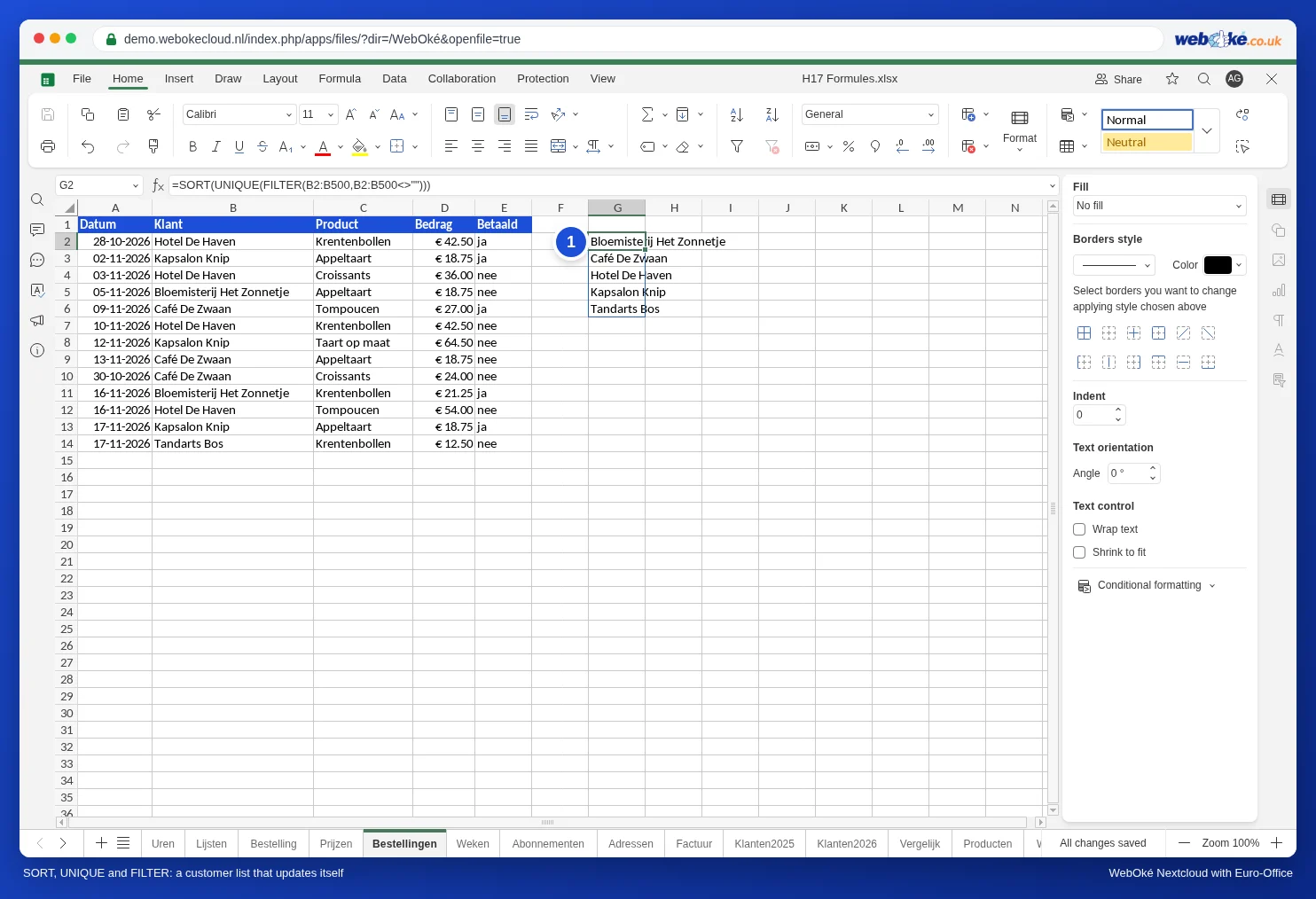
When an order comes in from a new customer, such as Tandarts Bos in row 14, that customer appears in the right place in the list straight away. To change the list, edit the formula in the first cell, G2.
All outstanding orders this month
FILTER can also return entire rows, with several conditions:
=FILTER(A2:D500,(E2:E500="nee")*(A2:A500>=EOMONTH(TODAY(),-1)+1),"nothing outstanding")
- The first part is what you want to see: columns A to D.
- The second part contains the conditions. Each condition goes in brackets. A * between them means and, a + means or.
- EOMONTH(TODAY(),-1)+1 is the first day of this month.
- The third part is the text to show if there are no results.
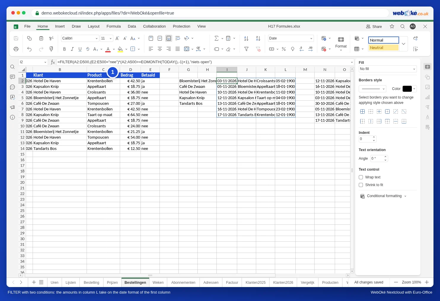
Please note: the result doesn't take over the formatting of your list. The amounts usually get the General format: €64.50 is shown as 64.5. Sometimes the whole result gets the format of the first column and the amounts are shown as dates, as in the image: 36.00 then becomes 05/02/1900. In either case, select the column with amounts in the result and choose the Currency or Number format yourself (see Formatting numbers, dates and currency).
Sorting and choosing columns
- By amount, highest first: =SORT(FILTER(A2:D500,E2:E500="nee"),4,-1). The 4 is the fourth column of the result, and -1 means descending.
- Sorting by a column you don't display: =SORTBY(FILTER(B2:B500,E2:E500="nee"),FILTER(D2:D500,E2:E500="nee"),-1) returns only the customer names, sorted by amount.
- Only customer and amount: =CHOOSECOLS(FILTER(A2:D500,E2:E500="nee"),2,4).
Tip: in the demo, the order of an existing =SORT(FILTER(...),4,-1) got mixed up after a new order was added below the list. A formula you enter after adding the order does sort correctly. So check the order whenever rows have been added. If it's wrong, enter the formula again: click the cell with the formula, press F2 and then Enter.
Something is in the way
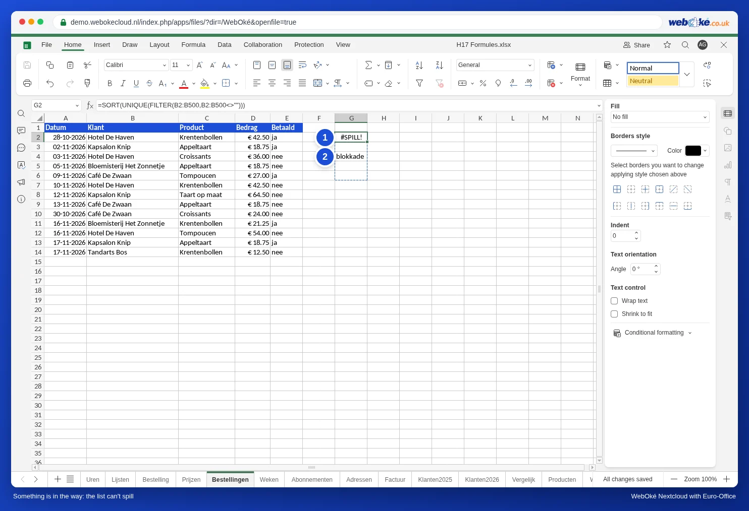
If a cell where the result needs to go already contains something, the list can't spill. In Excel, you then see the #SPILL! error. Euro-Office leaves the cell with the formula empty instead; click it and you'll see a dotted line around the area where the result wants to go. Clear the cells in that area and the list appears immediately. So keep some space free below and next to a formula like this.
Calculating with whole columns in one formula
Some formulas calculate with an entire column at once, such as =SUM(D2:D13*(E2:E13="nee")): the total amount of all orders that haven't been paid yet, 258.50 in this case. In Euro-Office, a formula like this works with a simple Enter. However, formulas that use IF over a whole column inside another function, such as =LARGE(IF(B2:B37="Pie",C2:C37),1), aren't calculated correctly by Euro-Office with a simple Enter: you get #NUM! or a wrong number. Finish a formula like this with Ctrl+Shift+Enter. The formula then gets curly brackets {…} and returns the correct result. Often you can do without IF and use FILTER instead: =LARGE(FILTER(C2:C37,B2:B37="Pie"),1).
What isn't possible
- LET and LAMBDA, and the functions built on them such as BYROW, MAP and GROUPBY, aren't supported in Euro-Office. An Excel file with these functions shows #NAME?. Use a helper column instead, or see Excel formulas with LET or LAMBDA: what to do in Euro-Office instead for alternatives.
- A colleague using Excel 2019 or older will see #NAME? for these functions.
Pitfalls
- Whole columns such as B:B make the formula slow. Choose a generous, fixed range such as B2:B500.
- No TRUE or FALSE without brackets in these formulas; use 1 and 0, or TRUE() and FALSE() (see Copying formulas from Excel: English function names and the comma).